

Top 80+ Machine Learning Interview Questions & Answers 2023

Are you willing to bag a job in machine learning and make the best of the opportunity? This blog will guide you on how to face the machine learning interview questions. The series of questions in this blog will help you understand the concept and answer the interview questions on machine learning with confidence and ease. The machine learning interview questions prepared in this blog are based on the study and experience gained from many reputed companies that choose to ask particular machine learning interview questions.
Let’s begin!
Prepare to brush up on your skills and have a confident machine-learning interview experience. So, what exactly does machine learning refers to? It is a process of developing the algorithm that trains the computer program to create statistical database patterns. Machine learning aims to identify the fundamental patterns of data and turn the data to define essential data insights.
For example, if we have an authentic dataset of actual sales figures, we can program the machine learning models to forecast or prefigure future sales reports.
Why is the Machine Learning trend on the high rise?
Machine learning is the core and imperative part of artificial intelligence. With basic machine learning algorithms, you can solve practical real-time problems. All the necessary information is extracted from the data and it is used to solve the issue and predict future figures. In recent times the statistics state that 80% of enterprises practicing machine learning and artificial intelligence have significantly progressed in the business and experienced immense financial growth. Machine Learning solves Real-World problems. Machine learning algorithms learn from the data, unlike the hard coding rule to solve the problem.
Many reputed companies welcome talent from the machine learning field; the growth is high and will continue to be in demand. The interviewers seek talent with sound knowledge of machine learning algorithms that can help automate the task without explicit programming. The candidate`s competence is tested by checking on his areas of expertise. So, prepare to leave a positive impact on the interviewers by clearing all the machine learning interview questions with confidence.
This comprehensive blog highlights the top 80+ machine learning interview questions in 2023.
Basic Machine learning interview questions
The basic machine learning interview questions cover a wide range of machine learning questions that will prove very beneficial for the candidate to present the machine learning concept and basic machine learning algorithm.
1. What is Machine Learning?
This is one of the basic machine learning interview questions so specify that machine learning is a type of artificial intelligence that allows computer systems to learn from data, without being explicitly programmed. It involves building models that can recognize patterns in the data and make predictions or decisions based on those patterns.

2. What are the stages of building a Machine Learning model?
The stages of building a machine learning model include:
- Collecting and preprocessing the data
- Splitting the data into training, validation, and test sets
- Choosing an appropriate model and training it on the training data
- Evaluating the model on the validation data and tuning the model's hyper-parameters
- Evaluating the final model on the test data
3. What is the difference between inductive and deductive learning?
Inductive learning involves learning from specific examples and making generalizations based on those examples. Deductive learning involves starting with general rules or principles and applying them to specific cases.
4. What is the difference between supervised, unsupervised, and reinforcement learning?
Keep a simple approach while answering this machine learning interview question, you can state that supervised learning involves training a model on labeled data, where the correct output is provided for each example in the training set. Unsupervised learning involves training a model on unlabeled data, where the model must find patterns in the data on its own.
Reinforcement learning involves training a model to make decisions in an interactive environment, where the model receives rewards or punishments based on its actions.
5. Out of model accuracy and performance which one is more important?
It depends on the context and the goals of the model. Accuracy is more important when the consequences of making a mistake are high, such as in medical diagnosis or financial prediction. Performance is more important when the model needs to make decisions in real-time, such as in a self-driving car or a recommendation system.
6. What is Bias- Variance tradeoff in Machine Learning?
The bias-variance tradeoff in machine learning refers to the tradeoff between the model’s ability to fit the training data well (low bias) and the model's ability to generalize to new data (low variance). A model with high bias will underfit the training data, while a model with high variance will overfit the training data.
7. Why do we need validation and test datasets?
Validation and test datasets are needed to evaluate the performance of a machine learning model. The validation set is used to tune the model’s hyper-parameters and evaluate its performance on unseen data. The test set is used to evaluate the final model's performance on completely unseen data.
8. What is the difference between Parametric and Non-parametric Models?
Parametric models make assumptions about the form of the underlying data distribution. Non-parametric models do not make assumptions and can be more flexible, but may also be more prone to over-fitting.
9. What are hyper-parameters, and how are they different from parameters?
Hyper-parameters are the parameters that control the behavior of a machine learning model, such as the learning rate or the number of hidden units in a neural network. They are set by the practitioner and are not learned from the data during training. Parameters are the values that are learned from the data during training.
10. What is Heteroscedasticity?
The variance of the error terms in a model that is not constant is known as heteroscedasticity. This can cause problems when estimating the model's parameters, as the assumptions of some estimation methods may not hold.
11. How can one determine which algorithm to be used for a given dataset?
There are several factors to consider when choosing an algorithm for a given dataset including the size and complexity of data, the type of task (classification, regression), and the desired level of interpretability. It is suggested to try several different algorithms and compare their performance on the data.
Machine learning Interview Questions On EDA & FE
This section covers the machine learning interview questions on EDA & FE techniques along with the normalization and standardization in machine learning. All points explained in very simple methods for candidate to understand well.
12. What are some EDA techniques?
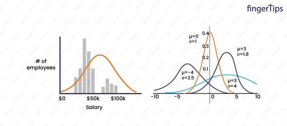
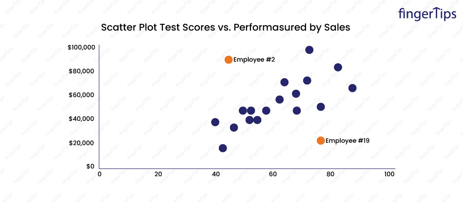
Exploratory Data Analysis techniques include visualizing data through plots and graphs, calculating summary statistics such as mean and standard deviation, and identifying patterns and trends in the data.
13. What is Cross-validation in Machine Learning?
Cross-validation is a method to evaluate the performance of a model by training it on a portion of the data and testing it on a different portion. This helps to prevent over-fitting, as the model is not just evaluated on the data it was trained on.
14. What are collinearity and multicollinearity?
Collinearity refers to the correlation between two or more predictor variables in a multiple regression model. Multicollinearity occurs when there is high collinearity among the predictor variables.
15. How to deal with multicollinearity?
There are several ways to deal with multicollinearity, including removing one or more of the highly correlated variables, using dimensionality reduction techniques such as principal component analysis (PCA), and adding regularization to the model.
16. What is the Variance Inflation Factor?
The Variance Inflation Factor is a measure of multicollinearity in a multiple regression model. It is calculated for each predictor variable and can be used to identify which variables may be causing multicollinearity.
17. What is PCA in Machine Learning?
Principal Component Analysis is a dimensionality reduction technique that projects the data onto a new set of orthogonal (uncorrelated) dimensions, known as principal components. We reduce number of dimensions and retain original variance as much as possible.
18. Why is rotation required in PCA? What will happen if the components are not rotated?
Rotation is required in PCA to ensure that the principal components are uncorrelated. If the components are not rotated, they may be correlated, which can affect the interpretation of the results.
19. What is meant by “Curse of Dimensionality”? List some ways to deal with it.
The "curse of dimensionality" refers to the challenges that arise when working with high-dimensional data, such as the need for a larger sample size and the difficulty in visualizing and interpreting the data. Some ways to deal with the curse of dimensionality include using dimensionality reduction techniques, such as PCA, and applying machine learning algorithms that are capable of handling high-dimensional data.
20. What is Dimensionality Reduction?
The process of reducing the number of dimensions (variables) in a dataset while preserving as much of the original information as possible is called Dimensionality reduction. This can be done for a variety of reasons, including improving model performance and reducing the complexity of the data.
21. What are some ways to Standardize Data?
Some ways to standardize data include scaling to have a mean of zero and a standard deviation of one and centering the data by subtracting the mean from each value.
22. What is the difference between Normalization and Standardization?
Normalization is the process of scaling the data to a specific range, such as [0, 1] or [-1, 1]. Standardization is the process of scaling the data to have a mean of zero and a standard deviation of one.
23. One-hot encoding increases the dimensionality of a dataset, but label encoding doesn’t. How?
One-hot encoding increases the dimensionality of a dataset by creating a new binary column for each unique category in a categorical variable. Label encoding does not increase the dimensionality of the dataset because it assigns a numerical value to each category in the variable, without creating new columns.
24. How can we handle an imbalanced dataset?
We can handle an imbalanced dataset by collecting more data, oversampling the minority class, under-sampling the majority class, and using algorithms that are specifically designed to handle imbalanced data.
25. What is a pipeline?
A pipeline is a series of steps that are performed on a dataset, like data preprocessing, feature selection, and model training. The goal is to automate the process and make it more efficient and reproducible.
Machine Learning Interview Questions Regression
In this machine learning interview question section you will discover all about regression. Many of your concepts on regression will be explained in detail.
26. What is Linear Regression in Machine Learning?
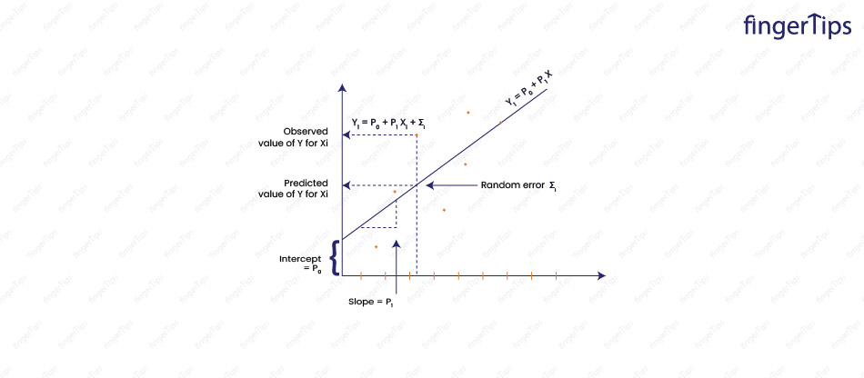
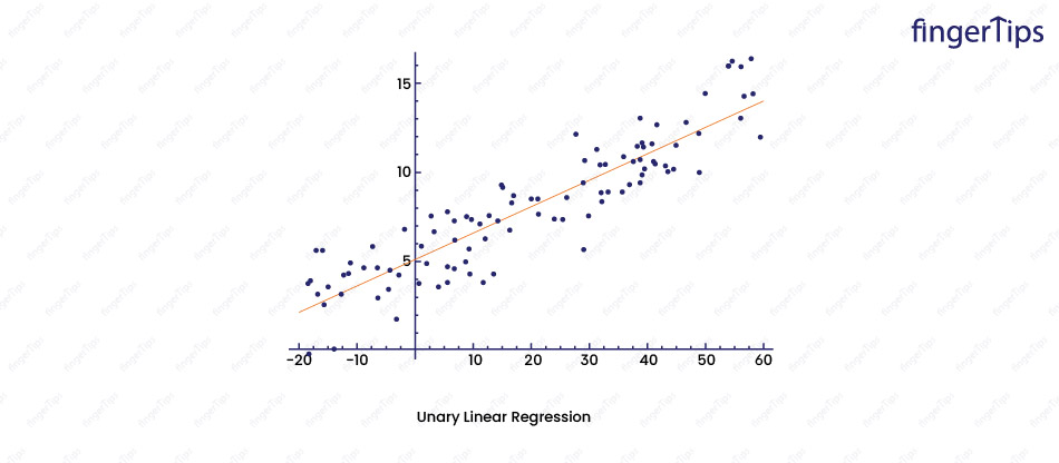
Linear regression is a statistical method used to model the linear relationship between a dependent variable and one or more independent variables. Wetry to find a straight line (or a hyper-plane in the case of multiple independent variables) that best fits the data and can be used to make predictions about the dependent variable.
27. What is the process of carrying out linear regression?
Be specific in explaining this machine learning interview question.
The process of carrying out linear regression involves the following steps:
- Collect and explore the data: This involves gathering the necessary data and performing exploratory data analysis.
- Prepare the data: This involves cleaning and preprocessing the data, such as handling missing values, scaling the variables, and splitting the data into training and test sets.
- Choose a model and train it: This involves selecting a suitable linear regression model (simple or multiple) and using the training data to estimate the model parameters.
- Evaluate the model: This involves using the test data to evaluate the performance of the model and assess its accuracy and predictive power.
- Fine-tune the model: The model can be fine-tuned by adjusting the parameters, adding or removing features, or using regularization.
- Make predictions: Once the model is trained and evaluated, it can be used to make predictions on new data.
28. Explain the difference between simple and multiple linear regression.
Simple linear regression involves only one independent variable, while multiple linear regression involves more than one.
Example: In simple linear regression, we try to predict the price of a house based on its size, while in multiple linear regression, we try to predict the price based on its size, location, number of rooms, etc.
29. Explain the concept of regularization and how it can be used in linear regression.
Regularization is a method to prevent over-fitting in linear regression by adding a penalty term to the objective function. The penalty term reduces the magnitude of the coefficients, which helps to reduce the complexity of the model and improve its performance.
There are two types of regularization used in linear regression:
- L2 or Ridge regularization: In this, we add a penalty term to the objective function that is proportional to the sum of the squares of the coefficients. The penalty term is controlled by a hyper-parameter called regularization strength or lambda. L2 regularization tends to produce models with small, non-zero coefficients, which can be useful for feature selection.
- L1 or Lasso regularization: In this, we add a penalty term to the objective function that is proportional to the sum of the absolute values of the coefficients. The penalty term is controlled by a hyper-parameter called regularization strength or alpha. L1 regularization tends to produce models with sparse coefficients, where many of the coefficients are exactly zero. This can be useful for feature selection and interpretation of the model.
Regularization is used to improve the performance of a linear regression model by reducing over-fitting. It is important to tune the regularization strength hyper-parameter to find the right balance between model complexity and error. Too much regularization can lead to under-fitting, while too little can lead to over-fitting.
30. What is the difference between Lasso and Ridge regression?
LASSO stands for Least Absolute Shrinkage and Selection Operator is a linear regression model that adds a penalty term to the objective function that is proportional to the sum of the absolute values of the coefficients:
Lasso objective function = MSE + alpha * ∑ |beta|
Where alpha is the regularization strength (a hyper-parameter) and beta is the coefficient for a feature.
Ridge regression adds a penalty term to the objective function that is proportional to the sum of the squares of the coefficients:
Ridge objective function = MSE + alpha * ∑ beta^2
31. When is ridge regression preferred over lasso?
Ridge regression and Lasso are both regularization techniques that can be used to prevent over-fitting in linear regression. Both methods add a penalty term to the objective function that reduces the magnitude of the coefficients, but they differ in the form of the penalty term.
Ridge regression is preferred when we want to include all the features in the model, but want to penalize large coefficients. This is useful when we have correlated features and want to include all of them in the model.
Lasso is preferred when we want to select a subset of the most important features and eliminate the less important ones. This is useful when we have a large number of features and want to reduce the complexity of the model.
It is suggested to try both Ridge and Lasso and compare the performance of the resulting models. The right regularization method will depend on the specific characteristics of the data and the goals of the analysis.
32. Which performance metrics can be used to estimate the efficiency of a linear regression model?
There are several metrics used to estimate the efficiency of a linear regression model:
- R-squared: The variance in the dependent variable which can be explained by the model. More the value of R-square, better the fit is.
- Mean squared error (MSE): The average squared difference between the predicted values and the true values. A lower MSE value indicates a better fit.
- Root mean squared error (RMSE): The square root of the MSE is more interpretable because it is in the same units as the dependent variable. RMSE value, better the fit is.
- Mean absolute error (MAE): This may be defined as the average absolute difference between predicted and true values. Lower the MAE value ,better the fit is.
- F-statistic: This statistic tests the hypothesis that the model is a significant improvement over a model with no independent variables. A higher F-statistic value indicates a better fit.
- Adjusted R-squared: An adjusted version of R-squared that takes into account the number of independent variables in the model. It is considered to be amore reliable metric than R-squared when we have a large number of independent variables.
No single metric is a perfect measure of model performance, and it's suggested to try multiple metrics to get a more complete picture of the model's efficiency.
33. Which performance metric is better R2 or adjusted R2?
R-squared and adjusted R-squared are both metrics that measure the proportion of the variance in the dependent variable that is explained by the model.
R2 = 1 - (SSE/SST)
SSE = sum of squared errors (i.e. the residual sum of squares)
SST= total sum of squares.
Adjusted R-squared is an adjusted version of R-squared that takes into account the number of independent variables in the model.
Adjusted R2 = 1 - (SSE/SST) * (n - 1)/(n - p - 1)
n = number of observations in the data set
p =the number of independent variables.
Both R-squared and adjusted R-squared are always between 0 and 1, and a higher value indicates a better fit.
Adjusted R-squared is generally considered to be a better metric because it is adjusted for the number of independent variables in the model and is therefore less prone to be overstated.
34. What is a Mean Squared error?
Mean squared error (MSE) is used to measure the quality of a linear regression model. It is the average squared difference between the predicted values (ŷ) and the true values (y) for all the observations in the data set:
MSE = (1/n) ∑ (y - ŷ)^2
n = number of observations.
It is always non-negative, the smaller the value, the better the model. A model with an MSE of zero is a perfect fit, while a model with a large MSE has a large average error.
MSE is sensitive to the scale of the variables, so it is useful to scale the variables before calculating the MSE. It is also sensitive to outliers, so it is important to identify and handle outliers before calculating the MSE.
35. What is the error term composed of in regression?
In a regression model, the error term also known as the residual is the difference between the predicted value of the dependent variable and the true value.
error = y - ŷ
y= true value of the dependent variable
ŷ = predicted value.
The error term is composed of two types of error:
- Irreducible error: Error that is inherent to the system being modeled and cannot be reduced by any means. For example, in the case of linear regression, the irreducible error is the error that is not explained by the independent variables.
- Reducible error: Error that is reduced by improving the model. It includes errors due to the limitations of the model (e.g. bias) and errors due to random noise in the data (e.g. variance).
36. How do you handle outliers in a linear regression model?
Outliers have a significant impact on the coefficients in a linear regression model, and sometimes even cause the model to be meaningless. One way to handle outliers is to simply remove them from the dataset before training the model. Another option is to use robust regression methods that are less sensitive to the presence of outliers.
37. How do you handle missing values in a linear regression model?
There are several approaches to handling missing values in a linear regression model:
- Deletion: Delete the rows with missing values
- Imputation: Impute the missing values using mean
- Prediction: Train a separate model to predict the missing values
Machine Learning Interview Questions Classification
Explore all about classification in this machine-learning question list.
38. Explain Logistic Regression
Logistic regression is a supervised learning algorithm used for classification problems. It takes a set of input features and makes predictions about the likelihood of an event occurring. The predicted probability is transformed into a binary prediction using a threshold.
For example, if the predicted probability is greater than 0.5, the instance is classified as belonging to the positive class, and if it is less than 0.5, the instance is classified as belonging to the negative class.
The logistic function, which is used to predict the probability, is defined as follows:
p = 1 / (1 + exp(-z))
z = linear combination of the input features and the model weights
exp = exponential function.
Logistic regression is used for binary classification, where the goal is to predict one of two classes, or for multiclass classification, where the goal is to predict one of more than two classes.
39. Logistic regression is a classification technique and not a regression, why? Name the function it is derived from.
Logistic regression is a classification technique, not a regression as it is used to predict a class label and a continuous numeric output.
The name "logistic regression" can be misleading, as it is a classification algorithm and not a regression algorithm.
It is called "logistic" because it uses the logistic function (also known as the sigmoid function) to predict the probability that an instance belongs to a particular class.
The logistic function maps any real-valued number to a value between 0 and 1, which can be interpreted as a probability, and thus logistic regression is used for classification tasks.
40. Can logistic regression be used for classes of more than 2?
Yes, logistic regression can be used for multiclass classification tasks.
In the standard logistic regression, we predict the probability that an instance belongs to a particular class. The class with the highest predicted probability is then chosen as the predicted class. This is known as one-versus-all (OvA) classification or multiclass logistic regression.
For example, wehave a dataset with 3 classes: “good”, “better”, and “best”. To perform multiclass logistic regression using the OvA method, we train three separate binary classifiers, one for each class:
- Classifier 1: good versus not good
- Classifier 2: better versus not better
- Classifier 3: best versus not best
To classify a new instance, we apply all three classifiers to the instance and choose the class with the highest predicted probability.
There are other approaches as well to multiclass logistic regression, such as one-versus-one (OvO) classification, which involves training a separate binary classifier for each pair of classes.
41. How would you evaluate a logistic regression model?
There are several ways to evaluate the performance of a logistic regression model:
- Accuracy: It is the proportion of correct predictions made by the model. It is calculated as the number of true positives and true negatives divided by the total number of instances. Accuracy can be misleading if the class distribution is imbalanced.
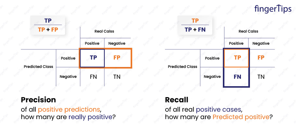
- Precision: It is the measure of the proportion of correct positive predictions. It is calculated as the number of true positives divided by the total number of positive predictions. Precision is useful for situations where false positives are more costly than false negatives.
- Recall: It is a measure of the proportion of actual positive instances that are correctly predicted by the model. Recall is number of true positives divided by the total number of actual positive instances. The recall is useful for situations where false negatives are more costly than false positives.
- F1 score: It is the harmonic mean of precision and recall, and is a good balance between the two. It is calculated as the harmonic mean of precision and recall, and is defined as F1 = 2 * (precision * recall) / (precision + recall)
- AUC-ROC: The AUC-ROC stands for the area under the receiver operating characteristic curve and is a metric that measures the ability of the model to distinguish between positive and negative classes. It is calculated by plotting the true positive rate against the false positive rate at various classification thresholds. A model with a high AUC-ROC score can correctly classify positive and negative instances more often than a model with a low AUC-ROC score.
42. Explain false negative, false positive, true negative, and true positive with an example.
- False negative: When a test incorrectly indicates that a condition is not present when it actually is present.
For example, if a medical test for a particular disease returns a negative result, but the patient actually has the disease, this is a false negative. - False positive: When a test incorrectly indicates that a condition is present when it actually is not present.
For example, if a pregnancy test returns a positive result, but he is not actually pregnant, this is a false positive. - True negative: When a test correctly indicates that a condition is not present.
For example, if a medical test for a particular disease returns a negative result, and the patient does not actually have the disease, this is a true negative. - True positive: When a test correctly indicates that a condition is present.
For example, if a pregnancy test returns a positive result, and the person is actually pregnant, this is a true positive.
43. What do you understand by Precision and Recall?
Precision and recall are two evaluation metrics to measure the accuracy of a classifier. For example, a binary classifier predicts whether an instance belongs to one of two classes (e.g., "positive" or "negative").
- Precision: This is the measure of the proportion of positive predictions that are actually correct. Number of true positives divided by the total number of positive predictions is called Precision. For example, if a classifier makes 100 positive predictions and 70 of them are correct, its precision is 70%.
- Recall: This is a measure of the proportion of actual positive instances that are correctly predicted by the classifier. Number of true positives divided by the total number of actual positive instances is known as Recall. For example, if there are 100 actual positive instances and the classifier correctly identifies 70 of them, its recall is 70%.
Both precision and recall are important in different situations.
For example, in a medical diagnosis setting, it is generally more important to have high recall (i.e., to minimize the number of false negatives, or missed diagnoses) even if it means accepting a higher number of false positives (incorrect diagnoses).
Whereas, in a spam filtering setting, it is generally more important to have high precision (i.e., to minimize the number of false positives, or non-spam emails that are classified as spam) even if it means accepting a higher number of false negatives (spam emails that are not detected).
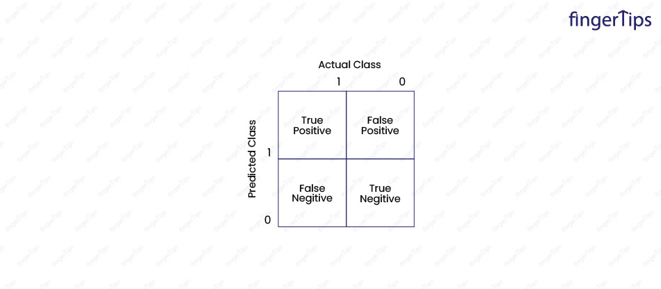
44. What is a Confusion Matrix?
A table used to evaluate the performance of a classifier is known as Confusion Matrix. The rows of the confusion matrix correspond to the actual classes of the instances, and the columns correspond to the predicted classes. The confusion matrix contains counts or proportions of the instances in each category.
|
|
Predicted Positive |
Predicted Negative |
|
Actual Positive |
True Positive (TP) |
False Negative (FN) |
|
Actual Negative |
False Positive (FP) |
True Negative (TN) |
The counts in the confusion matrix can be used to compute various evaluation metrics, such as precision, recall, and accuracy.
- Regularization: A technique used to prevent over-fitting by adding a penalty term to the objective function being optimized. The regularization term is a penalty on the L2 norm of the model weights, which is added to the negative log-likelihood loss. The strength of the regularization penalty is controlled by a hyper-parameter known as regularization strength, or lambda (λ).
- Learning rate: A hyper-parameter that controls the step size taken by the optimization algorithm during training. It determines how fast or slow the model learns from the training data. A smaller learning rate leads to a more accurate model, but it takes longer to train.
- Convergence tolerance: A hyper-parameter that determines the stopping criteria for the optimization algorithm. It is the maximum difference between the weights of two consecutive iterations that is allowed before the optimization is considered to have converged.
- Collect more data: This can help the classifier learn more about the less common classes and may improve its performance.
- Resample the data: By either over-sampling the underrepresented classes or under-sampling the overrepresented classes. -
- Use balanced class weights: Classifier like logistic regression supports class weights, which is used to adjust the impact of each class on the optimization process. We set higher weights for the underrepresented classes that help the classifier give more emphasis during training.
- Use a different evaluation metric: We may use an evaluation metric that is less sensitive to class imbalance, like the F1 score.
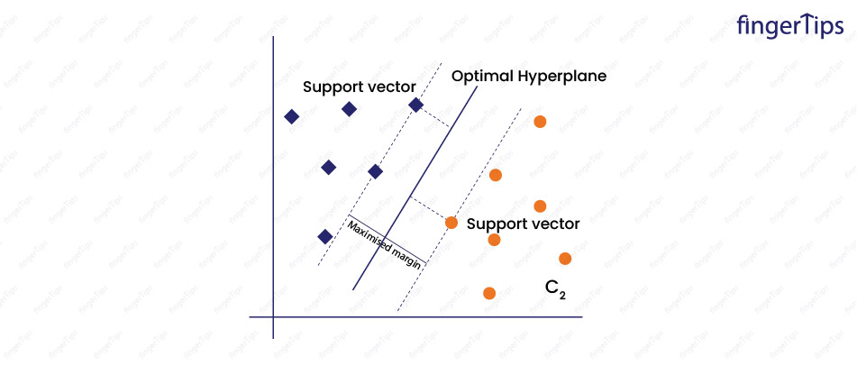
Machine Learning Interview Questions SVM
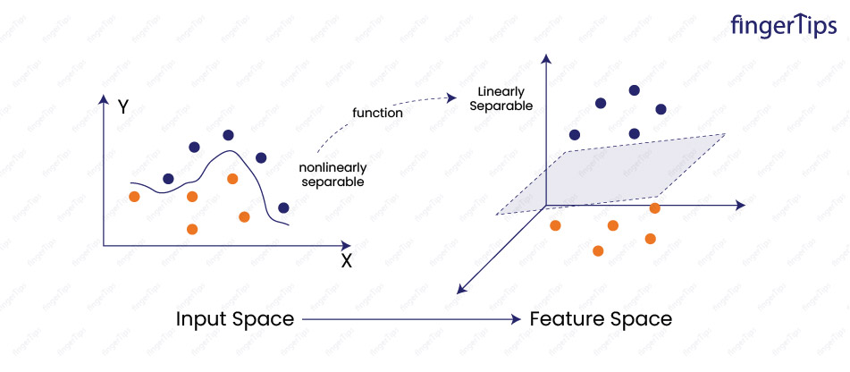
- Linear: The simplest kernel function which calculates the dot product between input data points.
- Polynomial: A non-linear kernel function that captures relationships between variables that are not linear.
- Radial Basis Function (RBF): A non-linear kernel function that is defined as the exponential of the negative Euclidean distance between the input data points.
- Sigmoid: A non-linear kernel function.
- Kernel: A hyper-parameter that is used to transform the data into a higher-dimensional space. Common kernel functions include linear, polynomial, radial basis functions, and sigmoid.
- Kernel coefficient: A hyper-parameter that is specific to the kernel function being used. For example, in the RBF kernel, the kernel coefficient is gamma, which determines the shape of the decision boundary.
- Regularization: A hyper-parameter that controls the complexity of the model. A higher value of the regularization means the model is less complex and more likely to generalize to unseen data, while a lower value means the model is more complex and less likely to generalize.
- Slack variables: In a soft margin SVM, these are hyper-parameters that control the degree of tolerance for misclassification. A higher value of the slack variables means the model is more tolerant of misclassified data points, while a lower value means the model is less tolerant.
- Under-sampling: It involves reducing the number of data points in the majority class to be equal to the number of data points in the minority class. This can be done by randomly selecting a subset of the majority class data points.
- Oversampling: It involves increasing the number of data points in the minority class by sampling with replacement from the minority class data points.
- SMOTE: Synthetic Minority Over-sampling Technique (SMOTE) is an oversampling method that generates synthetic data points for minority classes by interpolating between existing minority class data points.
- Adjust class weights: By setting the class_weight parameter to a "balanced" model gives more importance to the minority class data points.
- Use a different loss function: For example,the "hinge" loss function is more sensitive to the misclassification of the minority class data points, while the "squared hinge" loss function is more sensitive to the misclassification of the majority class data points.
- Accuracy
- Confusion matrix
- Precision
- Recall
- F1 score
- AUC-ROC curve
- Cross-validation
- It is sensitive to the selection of kernel and choice of hyper-parameters
- It is not well-suited for data sets with large numbers of features
- It is not robust to noise in data
- It is not easily interpretable
- It is not natively a probabilistic model
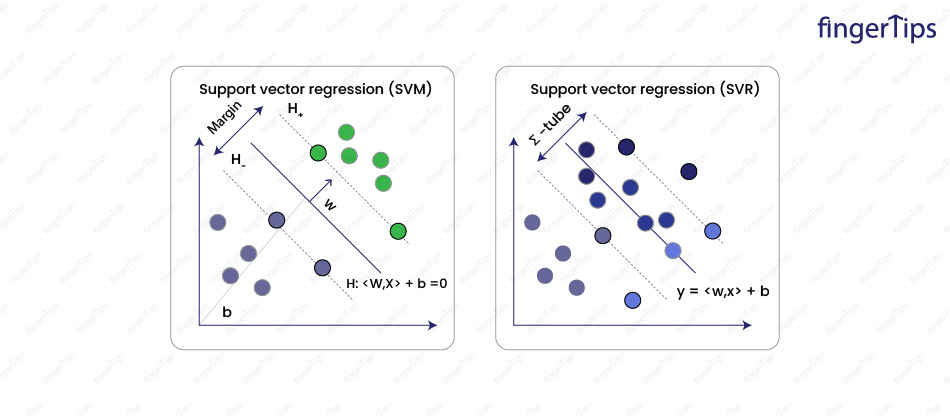
- Classification tasks
- Regression tasks
- Anomaly detection
- Feature selection
- Non-linear boundary decision
- Effective in high-dimensional spaces
- Robust to over-fitting
- Versatile
- Efficient
Machine Learning Interview Questions Naïve Bayes
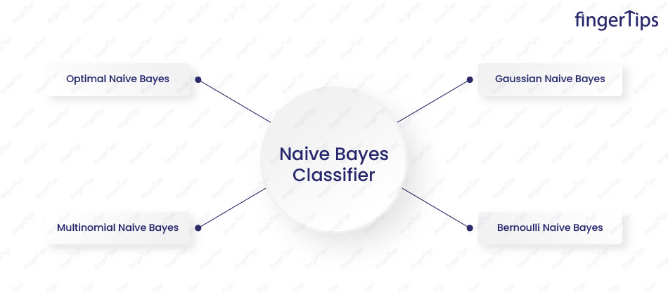
- Calculates the prior probability of each class.
- Calculate the likelihood of each feature occurring given each class.
- Multiply the prior probability of each class by the likelihood of each feature to get the posterior probability of each class.
- The class with the highest posterior probability is the predicted class.
- A simple and easy-to-implement algorithm.
- Fast and efficient, particularly for large datasets.
- Highly adaptive means it can adjust to changes in the distribution of the data.
- A probabilistic model means it outputs probabilities for each class label.
- Can achieve high accuracy even with a small amount of training data, and is often used as a baseline classifier.
- Spam filtering
- Document classification
- Sentiment analysis
- Medical diagnosis
- Fraud detection
- Weather prediction
Machine Learning Interview Questions KNN
- Euclidean distance: The straight-line distance between two points. It is calculated as the square root of the sum of the squares of the differences between the coordinates of the points.
- Manhattan distance: This is also known as the "taxi cab" distance because it is the distance a taxi cab would need to travel to get from one point to another following a grid-like pattern. It is calculated as the sum of the absolute differences between the coordinates of the points.
- Cosine similarity: This is used when data points are represented as vectors. It measures the similarity between two vectors by calculating the cosine of the angle between them.
- Jaccard index: This is used when the data points are set. It measures the similarity between two sets by calculating the size of the intersection divided by the size of the union.
- Minkowski distance: This is a generalization of the Euclidean and Manhattan distances. It is calculated as the sum of the absolute differences between the coordinates of the points raised to the power of p, where p is a positive integer.
- Mahalanobis distance: This is used to account for correlations in the data. It is calculated using the inverse of the covariance matrix of the data.
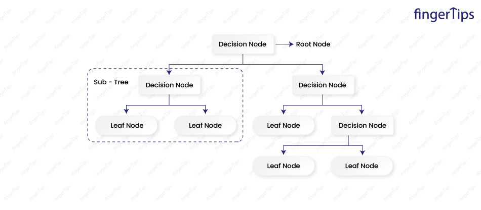
Machine Learning Interview Questions Decision Trees
- To prevent overfitting
- To improve interpretability
- To reduce computation time
- To improve prediction accuracy
- Maximum depth: Maximum number of nodes and the depth of the tree.
- Minimum samples per leaf: Minimum number of samples that must be present at a leaf node for the split to be considered.
- Minimum samples per split: Minimum number of samples that must be present at a node in for a split to be considered.
- Maximum features: Maximum number of features that can be considered when looking for the best split at each node.
- Maximum leaf nodes: Maximum number of leaf nodes that can be present in the tree. Smaller value results into a simpler tree.
- Criterion: Function that is used to evaluate the quality of a split.
- Splitter: The strategy that is used to select the split at each node.
- Class weight: Weight that is applied to each class in the training data.
- Presort: This determines whether or not to presort the data before building the tree.
- Easy to understand and interpret
- Can handle high-dimensional data
- Can handle both continuous and categorical data
- Fast to train and make predictions
- Can be prone to over-fitting
- May not be as accurate as other algorithms
- Can be sensitive to small changes in the data
- Can be unstablea. V
Machine Learning Interview Questions Ensemble Learning/Forests
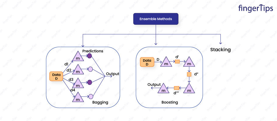
- Voting: Each base model makes a prediction, and the final prediction is made by taking the mode of the predictions for classification tasks orthe mean of the predictions for regression tasks.
- Averaging: Predictions of the base models are combined by taking the mean of the predictions in classification or regression tasks.
- Boosting: Base models are trained sequentially, correcting the mistakes made by the previous model. The final prediction is made by combining the predictions of all of the base models.
- Bagging: Multiple base models are trained on different subsets of input data. The final prediction is made by averaging the predictions made by the base models.
- Hard voting: Each base model makes a prediction and the final prediction is made by taking the mode of the predictions.
- Soft voting: Each base model makes a probability prediction, and the final prediction is made by taking the mean of the probability predictions.
Scenario Based Machine Learning Interview Questions
- Information about customers' subscription history like how long they have been a customer, how many subscriptions they have purchased in past, and whether they have consistently renewed their subscriptions in past.
- Demographic information such as age, gender, income level, and location.
- Usage data, including how often the customer uses the service and what features they use.
- Feedback or ratings provided by the customer as well as any interaction they had with customer support.